Custom Air Bubble Detector: Design and Application Guide

Engineers often treat air bubbles as minor annoyances until a batch fails or a pump runs dry. The reality? Even a microscopic bubble in the wrong place can compromise dosing accuracy, damage sensitive equipment, or trigger false alarms. Off-the-shelf detectors rarely match the unique geometries and fluid characteristics of custom systems. That’s why we created this design and application guide for custom air bubble detectors, drawing on real-world projects with Siansonic. Whether you’re wrestling with ultra-low flow rates, aggressive chemicals, or tight installation spaces, the following pages will show you how to specify, integrate, and validate a detector that actually fits your application.

Why Your Detector Misses Bubbles Under 0.5 mm

Most bubble detectors rely on either acoustic backscatter or optical extinction, and both methods struggle as diameters shrink below half a millimeter. The signal produced by a bubble scales roughly with its cross-sectional area—or worse, with the sixth power of radius in the Rayleigh scattering regime. By the time you're looking at a 0.4 mm bubble, the return is often buried in the electronic noise floor of the sensor. It's not that the bubble isn't there; it's that the detector literally cannot tell the difference between a faint echo and a random voltage spike.

Then there's the sampling problem. Even if a sensor has the raw sensitivity to spot a tiny bubble, it may only interrogate the flow at discrete intervals or over a narrow beam width. A 0.3 mm bubble moving at moderate flow velocity can cross the detection zone in a few milliseconds. If the system's dwell time or pulse repetition rate is too slow, the bubble simply slips through between measurements. This is especially common in clamp-on ultrasonic sensors where the acoustic path covers only a thin slice of the pipe volume.

Finally, many detectors are deliberately tuned to avoid false positives. Raising the trigger threshold keeps noise and particulate interference from generating alarms, but it also discards the weak signatures of sub-0.5 mm bubbles. Add smoothing filters or moving-average routines on top, and those already faint signals get averaged into oblivion. The result is a detector that reports clean liquid even when a stream of micro-bubbles is passing right through it.

Acoustic vs Optical: Pick Based on Tubing Material and Fluid Opacity

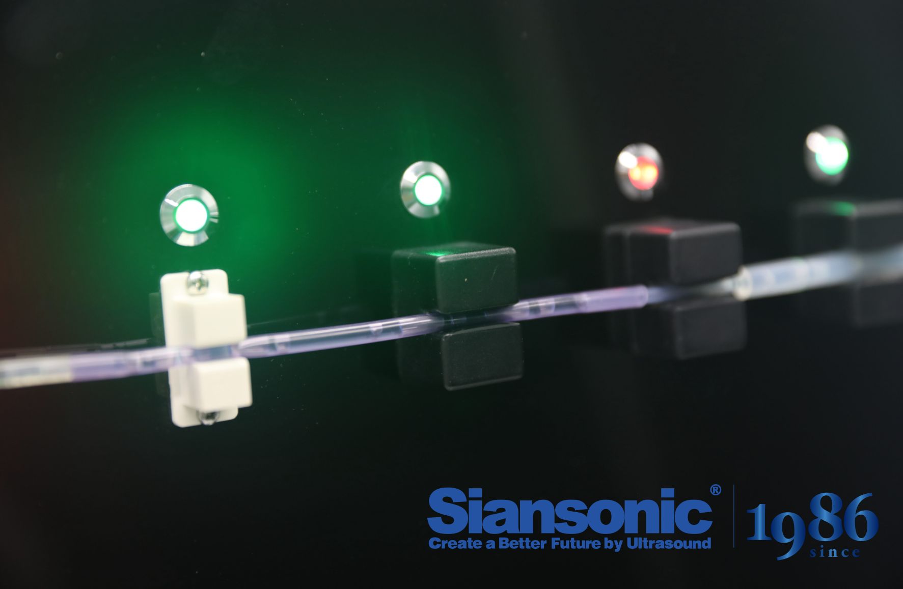
The choice between acoustic and optical sensing often comes down to what’s flowing through the tube and what the tube itself is made of. Acoustic methods rely on sound waves passing through the tubing wall and into the fluid, which means materials like soft silicone or Tygon that transmit vibrations well are natural partners. If your process runs opaque liquids—think inks, dairy, or sludge—acoustic sensors keep working without needing a clear window, since they don’t care about light penetration.

Optical sensors, on the other hand, demand a transparent or translucent tubing material so an infrared beam can reach the fluid. They excel with clear or slightly tinted liquids where you need to spot bubbles, sense liquid presence, or monitor color changes. But throw a dark, viscous fluid into the mix and optical detection can get unreliable fast, as the light gets absorbed or scattered before it returns a usable signal.

A practical rule: if your tubing is rigid PVC, glass, or another clear polymer and the fluid is see-through enough to read text through, optical is usually the simpler and cheaper route. If you’re dealing with blood, fermentation broth, or any fluid that would make a window useless, skip the optics and let acoustics do the heavy lifting—the tubing material just needs to carry a pulse, not a photon.

The Analog Chain: Turning Faint Echoes into Clean Triggers

A decent comparator does the heavy lifting, but only after the signal has been shaped enough to stop false triggers from the noise floor. I usually run the faint input through a high-gain stage with a gentle low-pass around 8 to 10 kHz first; that lifts the useful transient while shaving off the hiss that would otherwise make the threshold dance. Once the waveform is sitting just below the switching point, a small amount of positive feedback around the comparator turns a soft edge into a sharp, stable gate instead of a chattery burst.

The trick that gets overlooked is how you set the release. If the trigger decays too fast, a slightly weak hit can split into two pulses; too slow and fast phrases blur together. A simple diode and capacitor after the comparator gives a natural voltage decay, and adding a trimmer lets you match the decay to the source material rather than fighting it later. For acoustic drums, a few milliseconds of hold before release usually keeps the attack clean without turning rolls into mush.

Grounding and layout matter here more than in most line-level work. When the input is down in the tens of millivolts, any shared return path with a digital module can inject spikes that look exactly like the faint echo you are trying to capture. A separate analog ground, a small input transformer, or even just careful star wiring can make the difference between a chain that triggers on the real transient and one that responds to its own power supply.

Suppressing Roller Pump Artifacts Without Losing Sensitivity

Roller pump artifacts often appear as rhythmic spikes or baseline undulations that obscure genuine signals, especially in continuous flow systems. A common mistake is to apply aggressive low-pass filtering, which smears the waveform and buries small transient peaks. Instead of smoothing everything into a flat line, identify the pump's frequency signature and use a narrow notch filter or adaptive line cancellation only around those harmonics. This preserves the sharpness of real events while removing the mechanical noise that rides on top of them.

The key is to treat pump noise as a predictable, repeating interference rather than random drift. Triggered averaging synchronized to the pump cycle can subtract the artifact template from the raw trace, leaving the underlying signal intact. Because the pump stroke phase is constant relative to the roller position, this method works even when the signal amplitude is close to the noise floor. You retain full bandwidth for fast-changing peaks, unlike with broad filters that chop off high-frequency components indiscriminately.

Another effective route is to split the signal path early: one branch goes through a dedicated artifact reference channel that captures only the pump pulsation, while the other carries the mixed signal. By adaptively subtracting the reference after phase and gain alignment, you remove the mechanical component without touching signal dynamics. This dual-path approach avoids the trade-off between cleanliness and sensitivity that plagues one-size-fits-all filtering, making it ideal for trace-level detection in perfusion or chromatography systems.

A Reusable Test Setup for Verifying Detection Limits

A reusable test setup for verifying detection limits removes the need to rebuild the measurement chain for each new assay. The core idea is to keep the optical path, fluidic connections, and detector settings fixed while swapping only the sample introduction component. That way, any shift in the limit of detection can be traced back to a change in the assay itself, not to day-to-day differences in alignment or tubing length.

The setup usually includes a low-dead-volume flow cell, a calibrated injection loop, and a series of blank and low-concentration standards stored under inert gas. Running the sequence in triplicate and alternating blanks with spiked samples helps separate instrumental noise from true signal. A key detail is to use the same lot of reagents and to let the detector warm up for at least an hour before collecting data; otherwise, thermal drift can masquerade as a detection limit shift.

To confirm that the setup remains stable over time, it is useful to log the baseline noise and the slope of the calibration curve after each run. If the noise stays within a predefined band and the slope does not drift by more than a few percent, the reusable platform is considered fit for routine detection limit checks. This approach saves time and reduces the uncertainty that comes from assembling a fresh system for every verification.

Positioning Sensors Where Air Actually Collects in the Line

In most liquid handling systems, air does not disperse evenly the way one might hope. Instead, it tends to gather at high points, expansion sections, and areas where flow velocity suddenly drops. If a sensor is placed where the fluid moves smoothly and air is finely entrained, the reading will underestimate the actual gas volume present. To obtain meaningful measurements, you need to trace where bubbles actually linger during normal operation and shutdown.

Spotting air collection zones often starts with studying the pipe layout. The tops of vertical risers, dips in horizontal runs caused by inadequate support, and dead legs near pump suctions are common pockets where air accumulates. These areas usually show intermittent bubble release or pressure fluctuations. Placing sensors directly at these high points, or just downstream of them, captures far more air activity than picking a convenient location at random.

Sometimes a single sensor is not enough, because air collects in multiple separate spots, especially in branched networks or long transfer lines. Installing sensors at each known accumulation area and comparing their data gives a much clearer picture of how concentrated the air really is. This targeted arrangement requires extra installation effort, but it significantly improves the reliability of air detection and helps operators take venting or corrective action much sooner.

FAQ

Conclusion

Most custom detectors fail not from a lack of sensitivity but from overlooking where bubbles actually lodge and how tubing properties distort the signal. Bubbles under 0.5 mm rarely produce enough contrast for a basic threshold, especially in soft or opaque tubing. Acoustic sensors excel with clear or translucent lines and clean fluids, but they struggle when air pockets cling near tube walls or when fluid opacity scatters the beam. Optical sensors work better with rigid, light-transmissive tubing but can false-trigger on fluid color changes. Positioning matters just as much as the sensing principle: mounting the sensor at high points, near joints, or just after a pump where air collects dramatically improves detection. A detector that ignores these flow dynamics will keep missing the smallest bubbles no matter how advanced its electronics.

The analog front end must turn faint echoes or weak optical dips into clean, repeatable triggers without amplifying roller pump noise. A common mistake is using a fixed comparator threshold; instead, a band-pass filter tuned to the bubble's transit signature, followed by an envelope detector and a slow attack/fast release comparator, rejects periodic pump artifacts while preserving sensitivity. To verify real-world limits, build a reusable test rig with a syringe pump, a Y-connector for injecting known air volumes, and a calibrated capillary to confirm bubble diameter. Record the response for 0.3, 0.5, and 1.0 mm bubbles at different flow rates and tubing positions. Only after mapping these operating corners can you trust that the detector will alarm consistently—and not drive operators crazy with false positives.